Wednesday, March 31, 2010

General media

If observation is confined to regions sufficiently remote from a system of charges, a multipole expansion of the exact polarization density can be made. By truncating this expansion (for example, retaining only the dipole terms, or only the dipole and quadrupole terms, or etc.), the results of the previous section are regained. In particular, truncating the expansion at the dipole term, the result is indistinguishable from the polarization density generated by a uniform dipole moment confined to the charge region. To the accuracy of this dipole approximation, as shown in the previous section, the dipole moment density p(r) (which includes not only p but the location of p) serves as P(r).

At locations inside the charge array, to connect an array of paired charges to an approximation involving only a dipole moment density p(r) requires additional considerations. The simplest approximation is to replace the charge array with a model of ideal (infinitesimally spaced) dipoles. In particular, as in the example above that uses a constant dipole moment density confined to a finite region, a surface charge and depolarization field results. A more general version of this model (which allows the polarization to vary with position) is the customary approach using a electric susceptibility or electrical permittivity.

A more complex model of the point charge array introduces an effective medium by averaging the microscopic charges;[19] for example, the averaging can arrange that only dipole fields play a role. A related approach is to divide the charges into those nearby the point of observation, and those far enough away to allow a multipole expansion. The nearby charges then give rise to local field effects. In a common model of this type, the distant charges are treated as a homogeneous medium using a dielectric constant, and the nearby charges are treated only in a dipole approximation. The approximation of a medium or an array of charges by only dipoles and their associated dipole moment density is sometimes called the point dipole approximation, the discrete dipole approximation, or simply the dipole approximation.

Surface charge


Above, discussion was deferred for the leading divergence term in the expression for the potential due to the dipoles. This term results in a surface charge. The figure at the right provides an intuitive idea of why a surface charge arises. The figure shows a uniform array of identical dipoles between two surfaces. Internally, the heads and tails of dipoles are adjacent and cancel. At the bounding surfaces, however, no cancellation occurs. Instead, on one surface the dipole heads create a positive surface charge, while at the opposite surface the dipole tails create a negative surface charge. These two opposite surface charges create a net electric field in a direction opposite to the direction of the dipoles. This idea is given mathematical form using the potential expression above. The potential is


\frac {1}{4 \pi \varepsilon_0}\int   \boldsymbol{\nabla_{\boldsymbol {r_0}}\cdot}  \left( \boldsymbol{p} (  \boldsymbol{ r}_0 ) \frac {1}{|\boldsymbol r - \boldsymbol{r}_0|}  \right) d^3 \boldsymbol{ r}_0
=\frac {1}{4 \pi \varepsilon_0}\int   \frac  {\boldsymbol{p} ( \boldsymbol{ r}_0 )\boldsymbol{\cdot } d \boldsymbol  {A_0 } } {|\boldsymbol r - \boldsymbol{r}_0|} \ ,

with dAo an element of surface area of the volume. In the event that p(r) is a constant, only the surface term survives:

\phi  ( \boldsymbol{r} ) =\frac {1}{4 \pi \varepsilon_0}\int   \frac  {1}{|\boldsymbol r - \boldsymbol{r}_0|}\  \boldsymbol{p}  \cdot  d\boldsymbol{A_0} \ ,

with dAo an elementary area of the surface bounding the charges. In words, the potential due to a constant p inside the surface is equivalent to that of a surface charge σ = dA, which is positive for surface elements with a component in the direction of p and negative for surface elements pointed oppositely. (Usually the direction of a surface element is taken to be that of the outward normal to the surface at the location of the element.)

If the bounding surface is a sphere, and the point of observation is at the center of this sphere, the integration over the surface of the sphere is zero: the positive and negative surface charge contributions to the potential cancel. If the point of observation is off-center, however, a net potential can result (depending upon the situation) because the positive and negative charges are at different distances from the point of observation.[16] The field due to the surface charge is:

\boldsymbol E ( \boldsymbol{r} )  =-\frac  {1}{4 \pi \varepsilon_0} \boldsymbol{\nabla}_{\boldsymbol {r}}\int    \frac {1}{|\boldsymbol r - \boldsymbol{r}_0|}\  \boldsymbol{p}  \cdot  d\boldsymbol{A_0} \ ,

which, at the center of a spherical bounding surface is not zero (the fields of negative and positive charges on opposite sides of the center add because both fields point the same way) but is instead :[17]

\boldsymbol E =-\frac {\boldsymbol p}{3  \varepsilon_0}  \ .

If we suppose the polarization of the dipoles was induced by an external field, the polarization field opposes the applied field and sometimes is called a depolarization field.[18][19] In the case when the polarization is outside a spherical cavity, the field in the cavity due to the surrounding dipoles is in the same direction as the polarization.[20]

In particular, if the electric susceptibility is introduced through the approximation:

\boldsymbol{p(r)} = \varepsilon_0  \chi(\boldsymbol r ) \boldsymbol {E(r)} \ ,

then:

 \boldsymbol { \nabla \cdot p(r)}=\boldsymbol {  \nabla \cdot} \left( \chi \boldsymbol{ (r)}\varepsilon_0 \boldsymbol  {E(r)}\right) =-\rho_b \ .

Whenever χ (r) is used to model a step discontinuity at the boundary between two regions, the step produces a surface charge layer. For example, integrating along a normal to the bounding surface from a point just interior to one surface to another point just exterior:

\varepsilon_0 \hat{\boldsymbol n} \cdot \left(  \chi \boldsymbol{ (r_+)}\boldsymbol {E(r_+)}-\chi \boldsymbol{  (r_-)}\boldsymbol {E(r_-)}\right) =\frac{1}{A_n} \int d \Omega_n \  \rho_b = 0 \ ,

where An, Ωn indicate the area and volume of an elementary region straddling the boundary between the regions, and  \hat{\boldsymbol n} a unit normal to the surface. The right side vanishes as the volume shrinks, inasmuch as ρb is finite, indicating a discontinuity in E, and therefore a surface charge. That is, where the modeled medium includes a step in permittivity, the polarization density corresponding to the dipole moment density p(r) = χ(r)E(r) necessarily includes the contribution of a surface charge.[21][22][23]

It may be noted that a physically more realistic modeling of p(r) would cause the dipole moment density to taper off continuously to zero at the boundary of the confining region, rather than making a sudden step to zero density. Then the surface charge becomes zero at the boundary, and the surface charge is replaced by the divergence of a continuously varying dipole-moment density.

Electric dipole moment


In physics, the electric dipole moment is a measure of the separation of positive and negative electrical charges in a system of charges, that is, a measure of the charge system's overall polarity.

In the simple case of two point charges, one with charge + q and one with charge q, the electric dipole moment p is:

  \boldsymbol{p} = q \, \boldsymbol{d}

where d is the displacement vector pointing from the negative charge to the positive charge. Thus, the electric dipole moment vector p points from the negative charge to the positive charge. There is no inconsistency here, because the electric dipole moment has to do with orientation of the dipole, that is, the positions of the charges, and does not indicate the direction of the field originating in these charges.

An idealization of this two-charge system is the electrical point dipole consisting of two (infinite) charges only infinitesimally separated, but with a finite p = q d

Tuesday, March 30, 2010

Fission, high energy physics and condensed matter


n 1938, the German chemist Otto Hahn, a student of Rutherford, directed neutrons onto uranium atoms expecting to get transuranium elements. Instead, his chemical experiments showed barium A year later, Lise Meitner and her nephew Otto Frisch verified that Hahn's result were the first experimental nuclear fission. In 1944, Hahn received the Nobel prize in chemistry in which, despite the efforts of Hahn, the contributions of Meitner and Frisch were not recognized. as a product.

In the 1950s, the development of improved particle accelerators and particle detectors allowed scientists to study the impacts of atoms moving at high energies. Neutrons and protons were found to be hadrons, or composites of smaller particles called quarks. Standard models of nuclear physics were developed that successfully explained the properties of the nucleus in terms of these sub-atomic particles and the forces that govern their interactions.

Around 1985, Steven Chu and co-workers at Bell Labs developed a technique for lowering the temperatures of atoms using lasers. In the same year, a team led by William D. Phillips managed to contain atoms of sodium in a magnetic trap. The combination of these two techniques and a method based on the Doppler effect, developed by Claude Cohen-Tannoudji and his group, allows small numbers of atoms to be cooled to several microkelvin. This allows the atoms to be studied with great precision, and later led to the Nobel prize-winning discovery of Bose-Einstein condensation.

Historically, single atoms have been prohibitively small for scientific applications. Recently, devices have been constructed that use a single metal atom connected through organic ligands to construct a single electron transistor. Experiments have been carried out by trapping and slowing single atoms using laser cooling in a cavity to gain a better physical understanding of matter.

Subcomponents and quantum theory


The physicist J. J. Thomson, through his work on cathode rays in 1897, discovered the electron, and concluded that they were a component of every atom. Thus he overturned the belief that atoms are the indivisible, ultimate particles of matter.[23] Thomson postulated that the low mass, negatively-charged electrons were distributed throughout the atom, possibly rotating in rings, with their charge balanced by the presence of a uniform sea of positive charge. This later became known as the plum pudding model.

In 1909, Hans Geiger and Ernest Marsden, under the direction of physicist Ernest Rutherford, bombarded a sheet of gold foil with alpha rays—by then known to be positively charged helium atoms—and discovered that a small percentage of these particles were deflected through much larger angles than was predicted using Thomson's proposal. Rutherford interpreted the gold foil experiment as suggesting that the positive charge of a heavy gold atom and most of its mass was
concentrated in a nucleus at the center of the atom—the Rutherford model.
While experimenting with the products of radioactive decay, in 1913 radiochemist Frederick Soddy discovered that there appeared to be more than one type of atom at each position on the periodic table.[25] The term isotope was coined by Margaret Todd as a suitable name for different atoms that belong to the same element. J.J. Thomson created a technique for separating atom types through his work on ionized gases, which subsequently led to the discovery of stable isotopes.

Meanwhile, in 1913, physicist Niels Bohr suggested that the electrons were confined into clearly defined, quantized orbits, and could jump between these, but could not freely spiral inward or outward in intermediate states.[27] An electron must absorb or emit specific amounts of energy to transition between these fixed orbits. When the light from a heated material was passed through a prism, it produced a multi-colored spectrum. The appearance of fixed lines in this spectrum was successfully explained by these orbital transitions.[28]

Chemical bonds between atoms were now explained, by Gilbert Newton Lewis in 1916, as the interactions between their constituent electrons.[29] As the chemical properties of the elements were known to largely repeat themselves according to the periodic law,[30] in 1919 the American chemist Irving Langmuir suggested that this could be explained if the electrons in an atom were connected or clustered in some manner. Groups of electrons were thought to occupy a set of electron shells about the nucleus.[31]

In 1918, Rutherford discovered that the positive charge within every atom was always equal to an integer multiple of hydrogen nuclei, and deduced that all nuclei contained positively-charged particles called protons. The mass of the nucleus often exceeded this multiple, however, and speculated that the excess mass to be composed of neutrally-charged particles (neutrons).[citation needed]

The Stern–Gerlach experiment of 1922 provided further evidence of the quantum nature of the atom. When a beam of silver atoms was passed through a specially shaped magnetic field, the beam was split based on the direction of an atom's angular momentum, or spin. As this direction is random, the beam could be expected to spread into a line. Instead, the beam was split into two parts, depending on whether the atomic spin was oriented up or down.[32]

In 1926, Erwin Schrödinger, using Louis de Broglie's 1924 proposal that particles behave to an extent like waves, developed a mathematical model of the atom that described the electrons as three-dimensional waveforms, rather than point particles. A consequence of using waveforms to describe particles is that it is mathematically impossible to obtain precise values for both the position and momentum of a particle at the same time; this became known as the uncertainty principle, formulated by Werner Heisenberg in 1926. In this concept, for a given accuracy in measuring a position one could only obtain a range of probable values for momentum, and vice versa. This model was able to explain observations of atomic behavior that previous models could not, such as certain structural and spectral patterns of atoms larger than hydrogen. Thus, the planetary model of the atom was discarded in favor of one that described atomic orbital zones around the nucleus where a given electron is most likely to be observed.
The development of the mass spectrometer allowed the exact mass of atoms to be measured. The device uses a magnet to bend the trajectory of a beam of ions, and the amount of deflection is determined by the ratio of an atom's mass to its charge. The chemist Francis William Aston used this instrument to show that isotopes had different masses. The atomic mass of these isotopes varied by integer amounts, called the whole number rule.[35] The explanation for these different isotopes awaited the discovery of the neutron, a neutral-charged particle with a mass similar to the proton, by the physicist James Chadwick in 1932. Isotopes were then explained as elements with the same number of protons, but different numbers of neutrons within the nucleus.

Origin of scientific theory


Further progress in the understanding of atoms did not occur until the science of chemistry began to develop. In 1661, natural philosopher Robert Boyle published The Sceptical Chymist in which he argued that matter was composed of various combinations of different "corpuscules" or atoms, rather than the classical elements of air, earth, fire and water.[13] In 1789 the term element was defined by the French nobleman and scientific researcher Antoine Lavoisier to mean basic substances that could not be further broken down by the methods of chemistry.[14]

In 1803, English instructor and natural philosopher John Dalton used the concept of atoms to explain why elements always react in a ratio of small whole numbers—the law of multiple proportions—and why certain gases dissolve better in water than others. He proposed that each element consists of atoms of a single, unique type, and that these atoms can join together to form chemical compounds.[15][16] Dalton is considered the originator of modern atomic theory.[17]

Additional validation of particle theory (and by extension atomic theory) occurred in 1827 when botanist Robert Brown used a microscope to look at dust grains floating in water and discovered that they moved about erratically—a phenomenon that became known as "Brownian motion". J. Desaulx suggested in 1877 that the phenomenon was caused by the thermal motion of water molecules, and in 1905 Albert Einstein produced the first mathematical analysis of the motion.[18][19][20] French physicist Jean Perrin used Einstein's work to experimentally determine the mass and dimensions of atoms, thereby conclusively verifying Dalton's atomic theory.
in 1869, building upon earlier discoveries by such scientists as Lavoisier, Dmitri Mendeleevperiodic table.[22] The table itself is a visual representation of the periodic law which states certain chemical properties of elements repeat periodically when arranged by atomic number.
published the first functional

Atomism

The concept that matter is composed of discrete units and cannot be divided into arbitrarily tiny quantities has been around for millennia, but these ideas were founded in abstract, philosophical reasoning rather than experimentation and empirical observation. The nature of atoms in philosophy varied considerably over time and between cultures and schools, and often had spiritual elements. Nevertheless, the basic idea of the atom was adopted by scientists thousands of years later because it elegantly explained new discoveries in the field of chemistry.[5]

The earliest references to the concept of atoms date back to ancient India in the 6th century BCE,[6] appearing first in Jainism.[7] The Nyaya and Vaisheshika schools developed elaborate theories of how atoms combined into more complex objects.[8] In the West, the references to atoms emerged a century later from Leucippus, whose student, Democritus, systematized his views. In approximately 450 BCE, Democritus coined the term átomos (Greek: ἄτομος), which means "uncuttable" or "the smallest indivisible particle of matter". Although the Indian and Greek concepts of the atom were based purely on philosophy, modern science has retained the name coined by Democritus.[5]

Corpuscularianism is the postulate, expounded in the 13th-century by the alchemistPseudo-Geber (Geber),[9] that all physical bodies possess an inner and outer layer of minute particles or corpuscles.[10] Corpuscularianism is similar to the theory atomism, except that where atoms were supposed to be indivisible, corpuscles could in principle be divided. In this manner, for example, it was theorized that mercury could penetrate into metals and modify their inner structure.[11] Corpuscularianism stayed a dominant theory over the next several hundred years and was blended with alchemy by Robert Boyle and Isaac Newton in the 17th century.[10][12] It was used by Newton, for instance, in his development of the corpuscular theory of light.

Helium atom


The atom is a basic unit of matter consisting of a dense, central nucleus surrounded by a cloud of negatively charged electrons. The atomic nucleus contains a mix of positively charged protons and electrically neutral neutrons (except in the case of hydrogen-1, which is the only stable nuclideelectromagnetic force. Likewise, a group of atoms can remain bound to each other, forming a molecule. An atom containing an equal number of protons and electrons is electrically neutral, otherwise it has a positive or negative charge and is an ion. An atom is classified according to the number of protons and neutrons in its nucleus: the number of protons determines the chemical element, and the number of neutrons determine the isotope of the element.[1] with no neutron). The electrons of an atom are bound to the nucleus by the

The name atom comes from the Greek ἄτομος/átomos, α-τεμνω, which means uncuttable, or indivisible, something that cannot be divided further. The concept of an atom as an indivisible component of matter was first proposed by early Indian and Greek philosophers. In the 17th and 18th centuries, chemists provided a physical basis for this idea by showing that certain substances could not be further broken down by chemical methods. During the late 19th and early 20th centuries, physicists discovered subatomic components and structure inside the atom, thereby demonstrating that the 'atom' was divisible. The principles of quantum mechanics were used to successfully model the atom.[2][3]

Relative to everyday experience, atoms are minuscule objects with proportionately tiny masses. Atoms can only be observed individually using special instruments such as the scanning tunneling microscope. Over 99.9% of an atom's mass is concentrated in the nucleus,[note 1] with protons and neutrons having roughly equal mass. Each element has at least one isotope with unstable nuclei that can undergo radioactive decay. This can result in a transmutation that changes the number of protons or neutrons in a nucleus.[4] Electrons that are bound to atoms possess a set of stable energy levels, or orbitals, and can undergo transitions between them by absorbing or emitting photons that match the energy differences between the levels. The electrons determine the chemical properties of an element, and strongly influence an atom's magnetic properties.

Monday, March 29, 2010

Proton therapy

Description


Proton therapy is a type of external beam radiotherapy using ionizing radiation. During treatment, a particle accelerator is used to target the tumor with a beam of protons.[2][3] These charged particles damage the DNA of cells, ultimately causing their death or interfering with their ability to reproduce. Cancerous cells, because of their high rate of division and their reduced ability to repair damaged DNA, are particularly vulnerable to attack on their DNA.

Due to their relatively large mass, protons have little lateral side scatter in the tissue; the beam does not broaden much, stays focused on the tumor shape and delivers small dose side-effects to surrounding tissue. All protons of a given energy have a certain range; very few protons penetrate beyond that distance.[4] Furthermore, the dose delivered to tissue is maximum just over the last few millimeters of the particle’s range; this maximum is called the Bragg peak.[5]

To treat tumors at greater depths, the proton accelerator must produce a beam with higher energy, typically given in eV or electron volts. Tumors closer to the surface of the body are treated using protons with lower energy. The accelerators used for proton therapy typically produce protons with energies in the range of 70 to 250 MeV (Mega electron Volts: million electron Volts). By adjusting the energy of the protons during application of treatment, the cell damage due to the proton beam is maximized within the tumor itself. Tissues closer to the surface of the body than the tumor receive reduced radiation, and therefore reduced damage. Tissues deeper within the body receive very few protons so that the dosage becomes immeasurably small.[4]

In most treatments, protons of different energies with Bragg peaks at different depths are applied to treat the entire tumor. These Bragg peaks are shown as blue lines in the figure to the left. The total radiation dosage of the protons is called the Spread-Out Bragg Peak (SOBP), shown as a red line in figure to the left. It is important to understand that, while tissues behind or deeper than the tumor receive no radiation from proton therapy, the tissue in front of or shallower than the tumor receive radiation dosage based on the SOBP.

Proton–proton chain reaction

The proton–proton chain reaction is one of several fusion reactions by which stars convert hydrogen to helium, the primary alternative being the CNO cycle. The proton–proton chain dominates in stars the size of the Sun or smaller.

Overcoming electrostatic repulsion between two hydrogen nuclei requires a large amount of energy, and this reaction takes an average of more than 1010[citation needed] years to complete at the temperature of the Sun's core, because one of the protons has to beta decay via the weak interaction into a neutron during the brief moment of fusion. Because of the slow nature of this reaction the Sun is still shining; if it were faster, the Sun would have exhausted its hydrogen long ago.

In general, proton–proton fusion can occur only if the temperature (i.e. kinetic energy) of the protons is high enough to overcome their mutual Coulomb repulsion. The theory that proton–proton reactions were the basic principle by which the Sun and other stars burn was advocated by Arthur Stanley Eddington in the 1920s. At the time, the temperature of the Sun was considered too low to overcome the Coulomb barrier. After the development of quantum mechanics, it was discovered that tunneling of the wavefunctions of the protons through the repulsive barrier allows for fusion at a lower temperature than the classical prediction.

Subatomic particles


Modern particle physics research is focused on subatomic particles, including atomic constituents such as electrons, protons, and neutrons (protons and neutrons are actually composite particles, made up of quarks), particles produced by radioactive and scattering processes, such as photons, neutrinos, and muons, as well as a wide range of exotic particles.

Strictly speaking, the term particle is a misnomer because the dynamics of particle physics are governed by quantum mechanics. As such, they exhibit wave-particle duality, displaying particle-like behavior under certain experimental conditions and wave-like behavior in others (more technically they are described by state vectors in a Hilbert space; see quantum field theory). Following the convention of particle physicists, "elementary particles" refer to objects such as electrons and photons, it is well known that these "particles" display wave-like properties as well.

All the particles and their interactions observed to date can almost be described entirely by a quantum field theory called the Standard Model. The Standard Model has 17 species of elementary particles (12 fermions (24 if you count antiparticles separately), 4 vector bosons (5 if you count antiparticles separately), and 1 scalar boson, which can combine to form composite particles, accounting for the hundreds of other species of particles discovered since the 1960s. The Standard Model has been found to agree with almost all the experimental tests conducted to date. However, most particle physicists believe that it is an incomplete description of nature, and that a more fundamental theory awaits discovery. In recent years, measurements of neutrino mass have provided the first experimental deviations from the Standard Model.

Particle physics has had a large impact on the philosophy of science. Some particle physicists adhere to reductionism, a point of view that has been criticized and defended by philosophers and scientists. Part of the debate is described below

Neutron

The neutron is a subatomic particle with no net electric charge and a mass slightly larger than that of a proton. They are usually found in atomic nuclei. The nuclei of most atoms consist of protons and neutrons, which are therefore collectively referred to as nucleons. The number of protons in a nucleus is the atomic number and defines the type of element the atom forms. The number of neutrons is the neutron number and determines the isotope of an element. For example, the abundant carbon-12 isotope has 6 protons and 6 neutrons, while the very rare radioactive carbon-14 isotope has 6 protons and 8 neutrons.

While bound neutrons in stable nuclei are stable, free neutrons are unstable; they undergo beta decay with a mean lifetime of just under 15 minutes (885.7±0.8 s).[2] Free neutrons are produced in nuclear fission and fusion. Dedicated neutron sources like research reactors and spallation sources produce free neutrons for use in irradiation and in neutron scatteringchemical element, the free neutron is sometimes included in tables of nuclides. It is then considered to have an atomic number of zero and a mass number of one, and is sometimes referred to as neutronium. experiments. Even though it is not a

Hydron (chemistry)

In chemistry, hydron is the general name for the positive hydrogen H+ cation.

Hydron is the name for positive hydrogen ions without regard to nuclear mass, or positive ions formed from natural hydrogen (hydrogen that has not been subjected to isotope separation).

Traditionally, the term "proton" was and is used in place of "hydron", by itself and in many chemical terms. However, such usage is technically incorrect, as only 99.999% of natural hydrogen nuclei are protons; the rest are deuterons and rare tritons.

Hydron was located / identified by Walter Russell and documented in his 1926 book - "The Universal One"

Hydron was defined by IUPAC in 1988.[1][2]

The hydrated form of the hydrogen cation is the hydronium ion, H3O+(aq)

The negatively-charged counterpart of the hydron is the hydride anion, H-.

Hydrogen

Hydrogen

Hydrogen is the chemical element with atomic number 1. It is represented by the symbol H. With an atomic weight of 1.00794 u, hydrogen is the lightest and most abundant chemical element, constituting roughly 75 % of the Universe's elemental mass.[4] Stars in the main sequence are mainly composed of hydrogen in its plasma state. Naturally occurring elemental hydrogen is relatively rare on Earth.

The most common isotope of hydrogen is protium (name rarely used, symbol H) with a single proton and no neutrons. In ionic compounds it can take a negative charge (an anion known as a hydride and written as H), or as a positively-charged species H+. The latter cation is written as though composed of a bare proton, but in reality, hydrogen cations in ionic compounds always occur as more complex species. Hydrogen forms compounds with most elements and is present in water and most organic compounds. It plays a particularly important role in acid-base chemistryhydrogen atom has been of theoretical use. For example, as the only neutral atom with an analytic solution to the Schrödinger equation, the study of the energetics and bonding of the hydrogen atom played a key role in the development of quantum mechanics. with many reactions exchanging protons between soluble molecules. As the simplest atom known, the

Hydrogen gas (now known to be H2) was first artificially produced in the early 16th century, via the mixing of metals with strong acids. In 1766–81, Henry Cavendish was the first to recognize that hydrogen gas was a discrete substance,[5] and that it produces water when burned, a property which later gave it its name, which in Greek means "water-former". At standard temperature and pressure, hydrogen is a colorless, odorless, nonmetallic, tasteless, highly combustible diatomic gas with the molecular formula H2.

Industrial production is mainly from the steam reforming of natural gas, and less often from more energy-intensive hydrogen production methods like the electrolysis of water.[6] Most hydrogen is employed near its production site, with the two largest uses being fossil fuel processing (e.g., hydrocracking) and ammonia production, mostly for the fertilizer market.

Hydrogen is a concern in metallurgy as it can embrittle many metals,[7] complicating the design of pipelines and storage tanks.

Fermionic field


In quantum field theory, a fermionic field is a quantum field whose quanta are fermions; that is, they obey Fermi-Dirac statistics. Fermionic fields obey canonical anticommutation relations rather than the canonical commutation relations of bosonic fields.

The prominent example is the Dirac field which can describe spin-1/2 particles: electrons, protons, quarks, etc. The Dirac field is a 4-component spinor. It can also be described by two 2-component Weyl spinors. Spin-1/2 particles that have no antiparticles (possibly the neutrinos) can be described by a single 2-component Weyl spinor (or by a 4-component Majorana spinor, whose components are not independent).


Contents

  • 1 Basic properties
  • 2 Dirac fields
  • 3 See also
  • 4 References

1.Basic properties

Free (non-interacting) fermionic fields obey canonical anticommutation relations, i.e., involve the anticommutators {a,b} = ab + ba rather than the commutators [a,b] = abba of bosonic or standard quantum mechanics. Those relations also hold for interacting fermionic fields in the interaction picture, where the fields evolve in time as if free and the effects of the interaction are encoded in the evolution of the states.

It is these anticommutation relations that imply Fermi-Dirac statistics for the field quanta. They also result in the Pauli exclusion principle: two fermionic particles cannot occupy the same state at the same time.

2.Dirac fields

The prominent example of a spin-1/2 fermion field is the Dirac field (named after Paul Dirac), and denoted by ψ(x). The equation of motion for a free field is the Dirac equation,

where \gamma^{\mu}\, are gamma matrices and m is the mass. The simplest possible solutions to this equation are plane wave solutions, \psi_{1}(x) = u(p)e^{-ip.x}\, and \psi_{2}(x) = v(p)e^{ip.x}\,. These plane waveψ(x), allowing for the general expansion of the Dirac field as follows, solutions form a basis for the Fourier components of
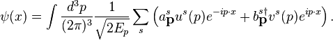
\psi(x) = \int \frac{d^{3}p}{(2\pi)^{3}}  \frac{1}{\sqrt{2E_{p}}}\sum_{s} \left( a^{s}_{\textbf{p}}u^{s}(p)e^{-ip \cdot x}+b^{s  \dagger}_{\textbf{p}}v^{s}(p)e^{ip \cdot x}\right).\,

The a\, and b\, labels are spinor indices and the s\, indices represent spin labels and so for the electron, a spin 1/2 particle, s = +1/2 or s=-1/2. The energy factor is the result of having a Lorentz invariant integration measure. Since \psi(x)\, can be thought of as an operator, the coefficents of its Fourier modes must be operators too. Hence, a^{s}_{\textbf{p}} and b^{s \dagger}_{\textbf{p}} are operators. The properties of these operators can be discerned from the properties of the field. \psi(x)\, and \psi(y)^{\dagger} obey the anticommutation relations

\{\psi_a(\textbf{x}),\psi_b^{\dagger}(\textbf{y})\} =  \delta^{(3)}(\textbf{x}-\textbf{y})\delta_{ab},

By putting in the expansions for \psi(x)\, and \psi(y)\,, the anticommutation relations for the coefficents can be computed.

\{a^{r}_{\textbf{p}},a^{s  \dagger}_{\textbf{q}}\} = \{b^{r}_{\textbf{p}},b^{s  \dagger}_{\textbf{q}}\}=(2 \pi)^{3} \delta^{3} (\textbf{p}-\textbf{q})  \delta^{rs},\,

In a manner analogous to non-relativistic annihilation and creation operators and their commutators, these algebras lead to the physical interpretation that a^{s \dagger}_{\textbf{p}} creates a fermion of momentum \textbf{p}\, and spin s, and b^{r \dagger}_{\textbf{q}} creates an antifermion of momentum \textbf{q}\, and spin r. The general field \psi(x)\, is now seen to be a weighed (by the energy factor) summation over all possible spins and momenta for creating fermions and antifermions. Its conjugate field, \bar{\psi} \  \stackrel{\mathrm{def}}{=}\  \psi^{\dagger} \gamma^{0}, is the opposite, a weighted summation over all possible spins and momenta for annihilating fermions and antifermions.

With the field modes understood and the conjugate field defined, it is possible to construct Lorentz invariant quantities for fermionic fields. The simplest is the quantity \overline{\psi}\psi\,. This makes the reason for the choice of \bar{\psi} = \psi^{\dagger} \gamma^{0}clear. This is because the general Lorentz transform on \psi\, is not unitary so the quantity \psi^{\dagger}\psi would not be invariant under such transforms, so the inclusion of \gamma^{0}\,Lorentz invariant quantity, up to an overall conjugation, constructable from the fermionic fields is \overline{\psi}\gamma^{\mu}\partial_{\mu}\psi. is to correct for this. The other possible non-zero

Since linear combinations of these quantities are also Lorentz invariant, this leads naturally to the Lagrangian density for the Dirac field by the requirement that the Euler-Lagrange equation of the system recover the Dirac equation.

\mathcal{L}_{D} = \bar{\psi}(i\gamma^{\mu}  \partial_{\mu} - m)\psi\,

Such an expression has its indices suppressed. When reintroduced the full expression is

\mathcal{L}_{D} =  \bar{\psi}_{a}(i\gamma^{\mu}_{ab} \partial_{\mu} -  m\mathbb{I}_{ab})\psi_{b}\,

Given the expression for ψ(x) we can construct the Feynman propagator for the fermion field:

 D_{F}(x-y) = \langle 0| T(\psi(x)  \bar{\psi}(y))| 0 \rangle

we define the time-ordered product for fermions with a minus sign due to their anticommuting nature

 T(\psi(x) \bar{\psi}(y)) \  \stackrel{\mathrm{def}}{=}\  \theta(x^{0}-y^{0}) \psi(x) \bar{\psi}(y)  -  \theta(y^{0}-x^{0})\bar\psi(y) \psi(x) .

Plugging our plane wave expansion for the fermion field into the above equation yields:

 D_{F}(x-y) = \int \frac{d^{4}p}{(2\pi)^{4}}  \frac{i(p\!\!\!/ + m)}{p^{2}-m^{2}+i \epsilon}e^{-ip \cdot (x-y)}

where we have employed the Feynman slash notation. This result makes sense since the factor

\frac{i(p\!\!\!/ + m)}{p^{2}-m^{2}}

is just the inverse of the operator acting on \psi(x)\, in the Dirac equation. Note that the Feynman propagator for the Klein-Gordon field has this same property. Since all reasonable observables (such as energy, charge, particle number, etc.) are built out of an even number of fermion fields, the commutation relation vanishes between any two observables at spacetime points outside the light cone. As we know from elementary quantum mechanics two simultaneously commuting observables can be measured simultaneously. We have therefore correctly implemented Lorentz invariance for the Dirac field, and preserved causality.

More complicated field theories involving interactions (such as Yukawa theory, or quantum electrodynamics) can be analyzed too, by various perturbative and non-perturbative methods.
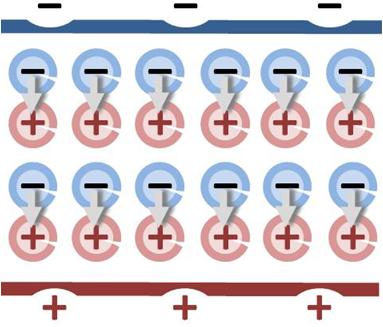